![]()
Admittedly, I am a bit worried about not utilizing my Excel skills each day. My old job pretty much required me to know a good deal of Excel. Excel was probably the one program aside from Outlook which I couldn’t live without.
Nowadays, it truly amazes me when I would run into co-workers who didn’t know how to use Excel for what it is, an easy way to collect and calculate data. You know that person, the one who sends you a spreadsheet that is busy as hell with colors, different size fonts, and worse yet – hard coded totals. WTH? Did the person actually break out a calculator (and I don’t even want to know if they used the calculator on the computer or an actual calculator). Ugh, you get what I mean.
So, I figured I would start putting out some quick how-to’s with Excel formulas. It gives me some Excel practice and can also inform others if they weren’t already aware of some Excel formulas. Now, I am starting with some of the basics. As time goes on I’ll expand and get into the more complicated formulas. But for the first few Excel posts, we’ll keep it pretty straight forward.
We’re using Excel 2007 at home. The formulas will work regardless of the version you’re running. So let’s get going…
=SUM
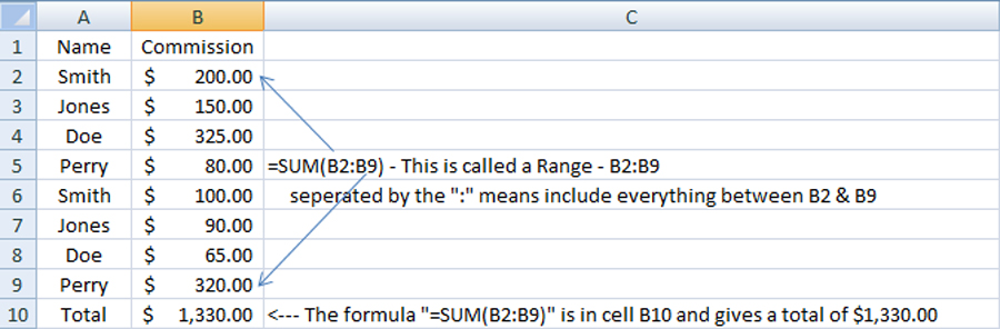
Let’s start with a straight forward one that will resolve you having to bring out your calculator just to add a few cells. Say you want to add a few rows of cells for commission totals. Using the =SUM formula, you can quickly add up the total. In the example below, typing “=SUM(B2:B9)”in cell B10 and pressing ENTER will give your total. It’s that easy. Keep in mind, there are several variations to these formulas which makes them even more powerful. =sumif for example. I’ll highlight those in future posts.
=COUNT
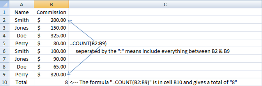
=COUNT is another simple one you can learn very quickly. Using the same example, if you’d like to count how many total commissions there are you can use the =COUNT formula. Sure, you could just count the number of lines, but the real beauty of the =COUNT formula is with it’s other versions : =COUNTIF and =COUNTA. =COUNT returns the number of cells that contain numbers. By typing in “=COUNT(B2:B9)” in cell B10 and pressing ENTER will give you the result “8” since there are a total of 8 cells that have something entered.
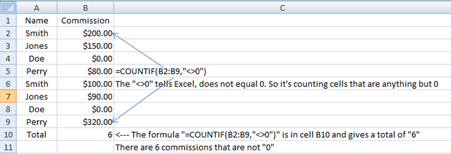
=COUNTIF – a more powerful version of the =COUNT formula. Changing a couple of the commissions to 0, say you want to count how many commissions there are which are not 0. Using the =COUNTIF function and some basic math greater than/less than (>/<) symbols, you can let Excel do the work for you. Typing in “=COUNTIF(B2:B9,”<>0″)” into cell B10 will result in a 6 since there are only “6” commissions that meets the does not equal 0 “<>0″ requirement.
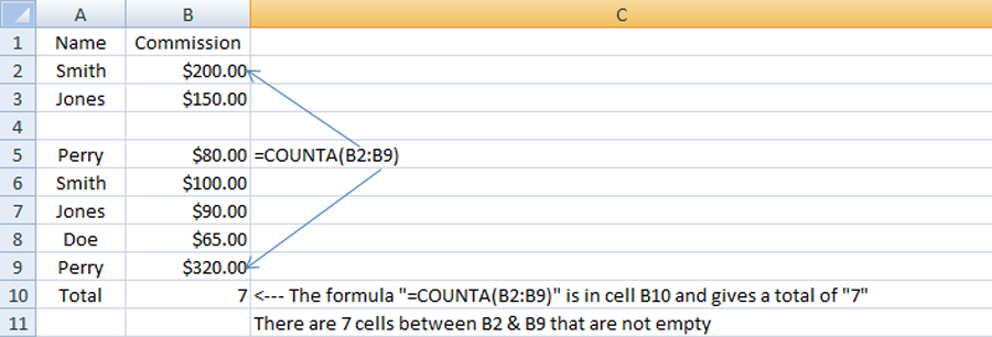
=COUNTA – another great version of the =COUNT formula. =COUNTA returns the number of cells that are not blank. Using this formula, Excel will count the range of cells which has anything in it, numbers or letters, just not blank cells. Typing in “=COUNTA(B2:B9)” and hitting ENTER, Excel will give you a response of “7” as there are 7 lines that contain data.
Okay, so that was 3 formulas for =COUNT, think of it as a bonus! Notice the difference between =COUNT and =COUNTA. =COUNT will give you the count of cells containing numbers. While =COUNTA will vie you the count of cells that contain anything but a blank.
=CONCATENATE
=CONCATENATE – That’s a fun word, concatenate. I tossed this one in there just because it’s fun to say and when this formula comes in handy, it really comes in handy. With =CONCATENATE you will merge multiple cells into one cell. For this example I’m going to use the formula wizard within Excel just to show you how that works. I don’t use the wizard because I’m already aware of how to put the structure of the formula together. But in Excel, there are several ways to complete any task. Once you become more comfortable with formulas, you’ll probably just start typing away. The wizard is handy in building formulas.
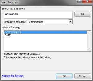
Using our example, let’s say there is now an additional column with the employees first name. Now you have the first name in one cell and the last in another.
Well, what if you’d like to have them both in one cell together. That’s where =CONCATENATE comes in handy. You may have noticed in Excel the blank bar with “fx” (function) proceeding it.
![]()
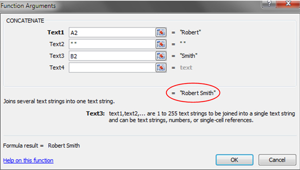
Making sure cell D2 is selected first, if you go go ahead and click that fx, the Insert Function wizard will launch. There is a search box that you can use to type the name of the function you want to insert. Here type in “concatenate” and hit ENTER or click GO, you’ll see it appear below. Click on it and hit OK.
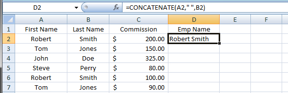
You’ll then see a new window, this is where you’ll be entering the arguments to let Excel know what things you want to put together into the cell. In the example, we want to join the contents in Column A with Column B in Column D. You’ll see the arguments listed as Text1 and Text2. If you click in the Text1 box, type in A2. After doing this Excel will let you know what you selected. In this case, “Robert”. When you click in Text2 you’ll notice Excel dropped in a new Text3 field. This will happen over and over again in case you have more arguments to enter. In our example, hit the SPACE bar once in the Text2 field and click over to Text3. Doing this will insert, yep you guessed it, a SPACE between the first and last names. Going to the Text3 box, type in B2 and “Smith” will appear. You can view the final outcome right under all the Text# fields, circled in RED below. Click on OK and you’re done!
After you click OK, you’ll see Excel completed the formula and now in cell D2 is “Robert Smith”. You have now merged two cells, it was that easy!
Here’s an Excel quick tip!
To copy formulas down quick and easy, let Excel do it for you. When the cell containing a formula is selected, like cell D2 in our example. Do you see how the bottom right-hand corner has kind of a black box in it?

Well, if you put your mouse over that black box you’ll notice it turns into a “+”, double-click when it changes to the “+” and Excel will copy the formula all the way to the last line of data for you! It will auto format the cells so the calculations apply to that next set of data. No more Copy & Paste, easy peasy. You could click & drag the “+” sign down to copy the formula.
To Bring It Home
The other great thing about Excel is there are typically 3 or 4 (or more) ways to do something. I only covered one shortcut in the examples above, in future posts I’ll cover many more. For the next Excel rundown, I’ll take on Pivot Tables. They’re crazy easy once you get used to them, and they are huge, HUGE in organizing data.
My dad had the kind of “suit and tie” career as I was growing up in the 70’s and 80’s. I can’t imagine how office work was done without Excel back then. Things that took what was probably days, only takes a couple moves and clicks of the mouse with Excel. I hope these few basic formulas will help those of you who are just getting into Excel.
Joe-
